pandas의 plot은 내부적으로 matplotlib.pyplot을 이용한다.
import numpy as npimport pandas as pdimport matplotlib.pyplot as pltdf1 = pd.DataFrame(np.random.randn(100, 3),
index=pd.date_range('1/1/2019', periods=100),
columns=['A', 'B', 'C']).cumsum()df1| A | B | C | |
|---|---|---|---|
| 2019-01-01 | -0.896370 | -1.962732 | 1.584821 |
| 2019-01-02 | -0.248402 | -3.101740 | 0.370419 |
| 2019-01-03 | 0.622560 | -3.979711 | 1.666569 |
| 2019-01-04 | 1.239019 | -3.443114 | 2.071264 |
| 2019-01-05 | 1.430470 | -2.562603 | 1.617184 |
| ... | ... | ... | ... |
| 2019-04-06 | -3.766329 | 1.028045 | -0.010892 |
| 2019-04-07 | -1.085759 | 0.827237 | -1.009741 |
| 2019-04-08 | -1.825895 | 0.261739 | -0.533710 |
| 2019-04-09 | -3.983964 | 1.580290 | -0.773006 |
| 2019-04-10 | -4.230757 | 0.500947 | -0.887232 |
100 rows × 3 columns
df1.plot()
plt.title('Pandas Plot Example')
plt.xlabel('Dates')
plt.ylabel('Data')
plt.show()
import seaborn as snstitanic = sns.load_dataset('titanic')titanic| survived | pclass | sex | age | sibsp | parch | fare | embarked | class | who | adult_male | deck | embark_town | alive | alone | |
|---|---|---|---|---|---|---|---|---|---|---|---|---|---|---|---|
| 0 | 0 | 3 | male | 22.0 | 1 | 0 | 7.2500 | S | Third | man | True | NaN | Southampton | no | False |
| 1 | 1 | 1 | female | 38.0 | 1 | 0 | 71.2833 | C | First | woman | False | C | Cherbourg | yes | False |
| 2 | 1 | 3 | female | 26.0 | 0 | 0 | 7.9250 | S | Third | woman | False | NaN | Southampton | yes | True |
| 3 | 1 | 1 | female | 35.0 | 1 | 0 | 53.1000 | S | First | woman | False | C | Southampton | yes | False |
| 4 | 0 | 3 | male | 35.0 | 0 | 0 | 8.0500 | S | Third | man | True | NaN | Southampton | no | True |
| ... | ... | ... | ... | ... | ... | ... | ... | ... | ... | ... | ... | ... | ... | ... | ... |
| 886 | 0 | 2 | male | 27.0 | 0 | 0 | 13.0000 | S | Second | man | True | NaN | Southampton | no | True |
| 887 | 1 | 1 | female | 19.0 | 0 | 0 | 30.0000 | S | First | woman | False | B | Southampton | yes | True |
| 888 | 0 | 3 | female | NaN | 1 | 2 | 23.4500 | S | Third | woman | False | NaN | Southampton | no | False |
| 889 | 1 | 1 | male | 26.0 | 0 | 0 | 30.0000 | C | First | man | True | C | Cherbourg | yes | True |
| 890 | 0 | 3 | male | 32.0 | 0 | 0 | 7.7500 | Q | Third | man | True | NaN | Queenstown | no | True |
891 rows × 15 columns
iris = sns.load_dataset('iris')iris| sepal_length | sepal_width | petal_length | petal_width | species | |
|---|---|---|---|---|---|
| 0 | 5.1 | 3.5 | 1.4 | 0.2 | setosa |
| 1 | 4.9 | 3.0 | 1.4 | 0.2 | setosa |
| 2 | 4.7 | 3.2 | 1.3 | 0.2 | setosa |
| 3 | 4.6 | 3.1 | 1.5 | 0.2 | setosa |
| 4 | 5.0 | 3.6 | 1.4 | 0.2 | setosa |
| ... | ... | ... | ... | ... | ... |
| 145 | 6.7 | 3.0 | 5.2 | 2.3 | virginica |
| 146 | 6.3 | 2.5 | 5.0 | 1.9 | virginica |
| 147 | 6.5 | 3.0 | 5.2 | 2.0 | virginica |
| 148 | 6.2 | 3.4 | 5.4 | 2.3 | virginica |
| 149 | 5.9 | 3.0 | 5.1 | 1.8 | virginica |
150 rows × 5 columns
iris.sepal_length[:20].plot(kind='line', rot=0)<matplotlib.axes._subplots.AxesSubplot at 0x1a25717a10>
iris.sepal_length[:20].plot.bar()<matplotlib.axes._subplots.AxesSubplot at 0x1a245dcfd0>
df2 = iris.groupby(iris.species).mean()df2| sepal_length | sepal_width | petal_length | petal_width | |
|---|---|---|---|---|
| species | ||||
| setosa | 5.006 | 3.428 | 1.462 | 0.246 |
| versicolor | 5.936 | 2.770 | 4.260 | 1.326 |
| virginica | 6.588 | 2.974 | 5.552 | 2.026 |
df2.plot.bar()<matplotlib.axes._subplots.AxesSubplot at 0x1a2460be50>
df2.T.plot.bar()<matplotlib.axes._subplots.AxesSubplot at 0x1a2470c490>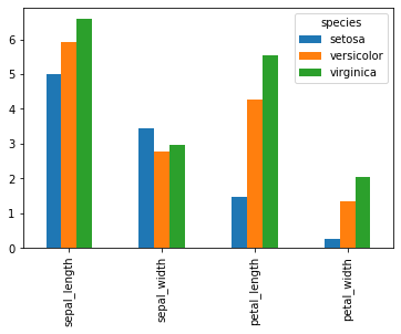
df3 = titanic.pclass.value_counts()
df3
3 491
1 216
2 184
Name: pclass, dtype: int64df3.plot.pie(autopct='%.2f%%')
plt.axis('equal')(-1.110415878418142, 1.100496015606113, -1.134350102435046, 1.112420061514539)
iris.plot.hist()<matplotlib.axes._subplots.AxesSubplot at 0x1a24bea850>
iris.plot.kde()<matplotlib.axes._subplots.AxesSubplot at 0x1a24d43050>
iris.plot.box()<matplotlib.axes._subplots.AxesSubplot at 0x1a24e3cb10>

iris.boxplot(by='species')array([[<matplotlib.axes._subplots.AxesSubplot object at 0x1a24d25590>,
<matplotlib.axes._subplots.AxesSubplot object at 0x1a24c16b90>],
[<matplotlib.axes._subplots.AxesSubplot object at 0x1a24c49dd0>,
<matplotlib.axes._subplots.AxesSubplot object at 0x1a24acbd90>]],
dtype=object)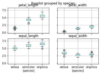
'분석 > 파이썬 Python' 카테고리의 다른 글
| Python : 순열검정 (비모수) (0) | 2024.01.27 |
|---|---|
| Python : 위도.경도로 TimeZone 구하기 (0) | 2020.03.10 |
| python : pd.to_numeric() VS astype(np.float64) (1) | 2019.11.27 |
| Python : Seaborn Visualization (0) | 2019.11.25 |
| Python : timedelta(months=3) 방법 (0) | 2019.11.12 |


